Why optimising the power grid actually matters
How carbon taxes, storage, and grid upgrades shape electricity costs and emissions, explored through an optimal power flow model that balances physics, policy, and practical optimisation.

Why optimising the grid matters?
Every time we turn on a kettle, plug in a laptop, or charge a car, we’re relying on one of the most complex systems in the country: the national electricity grid.
The grid stretches across thousands of kilometres, connecting power plants, substations, batteries, and homes. At any given moment, electricity must be generated, routed, and used in balance. Too much or too little, and the system fails.
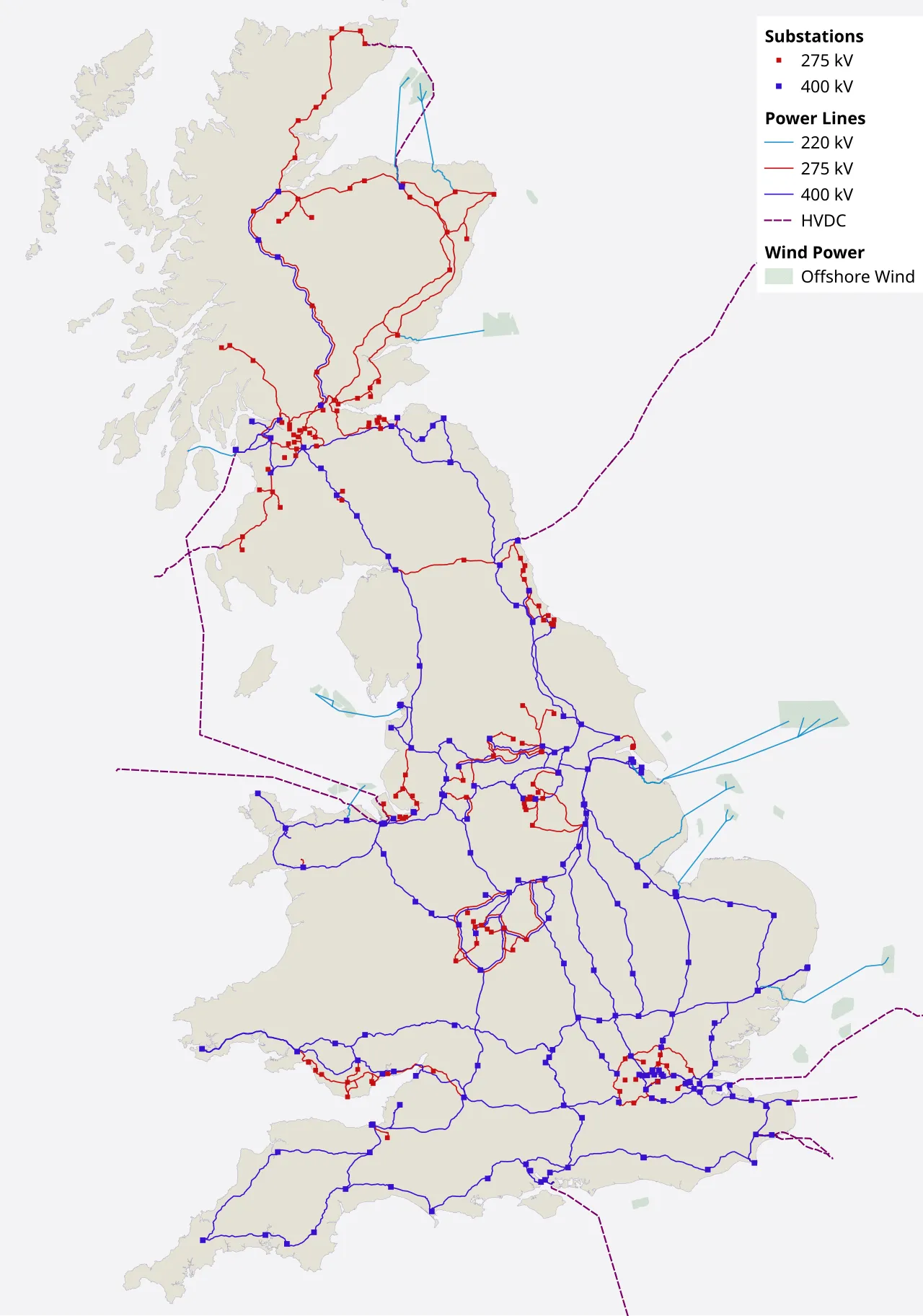
The structure of the UK National Grid, showing transmission lines and offshore wind links.
Behind the scenes, a constant stream of decisions is being made: which power stations should run, how much they should generate, where that electricity should go, and what it will cost. These decisions aren’t just driven by engineering. They’re shaped by market prices, regulations, and climate targets. And they have to be made in real time, every second of the day.
This is where Optimal Power Flow (OPF) comes in. It’s a mathematical framework that helps operators find the most efficient and cost effective way to run the grid, without violating physical or operational limits. It turns the chaos of the power system into something we can model, simulate, and optimise.
As the UK moves toward a net zero grid powered by wind, solar, and batteries, these models are becoming essential. Fossil fuels are predictable. Renewables are not. The better we can simulate and optimise the grid, the smoother and more affordable the transition will be.
In this post, I’ll walk through a simplified OPF model I built from scratch. It doesn’t capture every detail of the real grid, but it’s realistic enough to surface the key trade offs and behaviours. The model includes:
- a mix of generators, each with their own cost and emissions profile
- a basic transmission network with capacity constraints
- carbon pricing to reflect environmental costs
- storage systems that shift energy over time
- and Phase Angle Regulators (PARs) to control flow without building new lines
The goal is to explore questions that grid planners and policymakers are actively dealing with. Can carbon taxes alone drive down emissions? Are smart devices like PARs a cost effective alternative to new infrastructure? Where is the line between technical feasibility and economic efficiency?
Modelling approach
At first glance, modelling the power grid seems simple enough. A few power plants, some demand, a handful of cables. How hard can it be?
Turns out, even a simplified grid gets complex fast. It’s a system where physics, economics, policy, and time all collide. Every choice affects everything else. If the structure isn’t well thought out, the model quickly becomes unmanageable. But with the right design, it turns into a useful space where trade offs between cost, capacity, and emissions play out naturally.
The first decision was how to represent the grid. I followed the standard approach: a network of buses (nodes), connected by transmission lines, with generators, loads, and storage all plugged into those buses. This gives a clean structure for modelling flows, tracking demand, and spotting bottlenecks.
Next came power flow. Full AC models are accurate but nonlinear and heavy to compute. They’re great if you want realism down to the last volt, but not ideal if you’re also trying to solve an optimisation problem in a reasonable timeframe. So I went with the DC approximation. It’s a linear simplification that assumes small angle differences and ignores reactive power. While not perfect, it’s well suited to planning and dispatch problems. And much easier to work with too.
Then there’s the objective. The default was to minimise cost, a total generation cost plus a carbon tax. This setup lets the model balance cheap, dirty power against cleaner, more expensive alternatives. Later on, I also tested an emissions minimising version, just to see how different priorities shift the outcome.
The final step was to formalise the constraints. That meant turning all the engineering logic into actual equations. That’s where the real structure of the model began to take shape.
Mathematical structure
Once I had a clear mental picture of how I wanted the model to work, it was time to structure it. If the previous section was about the thinking behind the model, this one is about the doing. I’m going to lay out the actual components, how they connect, and what role each one plays in the optimisation puzzle.
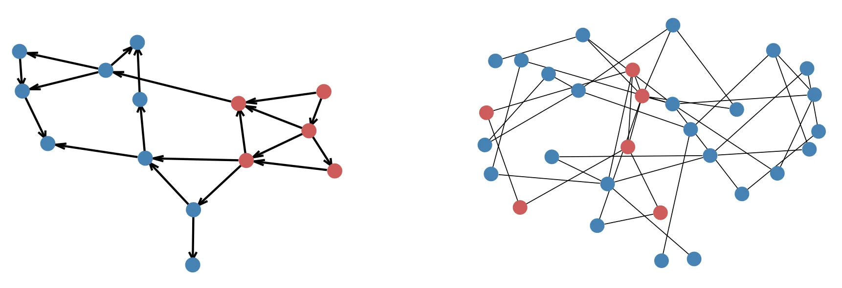
The graph representation of synthetic grids. Red and blue circles denote generator and load buses, respectively.
Sets and indices
At the heart of every optimisation model are sets. These are the building blocks that tell us what things we’re working with. In this case:
- : Set of generators. Each one has a cost, fuel type, and emissions profile.
- : Set of transmission lines. These connect nodes and carry flow.
- : Set of buses. Think of these as nodes or junction points in the grid.
- : Time periods. I modelled 24 hours in a day.
- : Fuel types. For example, gas, coal, or biomass.
- : Storage units. These can charge or discharge power.
This structure allows us to index everything properly. For example, means the power from generator during time .
Parameters
Parameters are the known facts, things the model doesn’t control. For example:
| Parameter | Description |
|---|---|
| Length of period | |
| Carbon tax in $/tonne of CO | |
| Power demand at bus in period | |
| Max power flow through line | |
| Max generation capacity of generator | |
| Bus/line incidence matrix element | |
| Generation cost for generator ($/MWh) | |
| Bus where generator is connected | |
| Reactance of line | |
| Efficiency of generator | |
| CO emissions per MWh for fuel | |
| Efficiency of storage unit | |
| Maximum energy storage capacity of unit | |
| Initial stored energy in storage | |
| Heat loss factor (if applicable) |
These parameters define the physical world, the cost structure, and the environmental impact, all of which the optimiser has to work with.
Decision variables
These are what the optimiser controls. They’re the knobs and switches it turns to find the optimal solution.
| Variable | Description |
|---|---|
| Power flow in line at time | |
| Power generated by generator at time | |
| Voltage phase angle at bus | |
| Power into (+ve) or out of (−ve) storage at time | |
| Energy level of storage at the start of period | |
| Phase angle regulator value for line (only if equipped) |
Objective function
The objective is simple in concept, but powerful in implication. We want to minimise total cost, where cost includes both operational cost and emissions cost.
The first term accounts for the direct cost of generating electricity. The second term adds a penalty proportional to carbon intensity, scaled by the generator’s efficiency and fuel type. This setup enables policy driven exploration, such as assessing the impact of increasing the carbon tax or comparing low carbon technologies under different incentive schemes.
Constraints to keep the model realistic
Constraints aren’t just rules for the sake of modelling. They’re the fundamental limits of how the grid works. Power doesn’t appear out of nowhere. Generators have output limits. Storage can’t recharge itself arbitrarily. These constraints reflect the physics of electricity, the technical limits of infrastructure, and the realities of policy, whether it’s carbon pricing, efficiency standards, or regulatory caps.
Constraints (1-2) balance supply and demand at each bus, (3) links phase angles to power flows, and (4-5) set limits on generation and transmission capacity. Storage is managed by (6-8), which control charging, discharging, and total energy volume. Constraints (9-16) apply to thermal storage, covering temperature limits, heat loss, and how energy evolves over time.
Implementing the model in Mosel Xpress
For this little project, I used Mosel Xpress, a solver native modelling language.
model OPF_with_storage
uses "mmxprs"
uses "mmsystem"
declarations
  nT: integer                         ! Number of periods
end-declarations

initialisations from "data.dat"
  nT
end-initialisations

declarations
  !! sets
  setG: set of string                 ! Set of generators
  setB: set of string                 ! Set of buses
  setL: set of string                 ! Set of lines
  setT = 1..nT                        ! Set of periods

  !! parameters
  Ht: integer                         ! Duration of period [h]
  tax: integer                        ! Carbon tax [$]
  PbtD: array(setT,setB) of real      ! Load in period  [GW]
  PlLplus: array(setL) of real        ! Maximum load in a line [GW]
  PgGplus: array(setG) of real        ! Maximum generation [GW]
  abl: array(setB,setL) of real       ! Element of bus/line
  CgG: array(setG) of real            ! Generation cost [$]
  betag: array(setG) of string        ! Bus to which generator is connected
  Xl: array(setL) of real             ! Reactance
  emissions: array(setG) of real      ! Emissions from fuel [tCO2/GWh]
  efficiency: array(setG) of real     ! Generator's efficiency

  !! variables
  pltL: array(setL, setT) of mpvar    ! Power flow in line l
  pgtG: array(setG, setT) of mpvar    ! Generation from generator g
  deltaB: array(setB, setT) of mpvar  ! Phase angle at bus b
end-declarations

!! function for cyclic model
function nxt(t,T:integer):integer
  returned:= t mod T + 1
end-function

!! declare pollution in period t
forall(t in setT) pollution(t):= sum(g in setG) Ht*(pgtG(g,t)*emissions(g))/efficiency(g)

!! objective function:
total_cost:= sum(g in setG, t in setT) CgG(g) * Ht * pgtG(g,t) + sum(t in setT) tax*pollution(t)
Mosel made it surprisingly smooth to translate the maths into code. Defining sets, parameters, and constraints felt natural, and it handled multi dimensional arrays, time loops, and conditional logic without much fuss. I was able to model multi period power flows, storage behaviour, and heat loss with minimal boilerplate, which kept things readable and easy to iterate on.
The built in integration with the Xpress solver was a bonus. I could focus on structure and logic instead of worrying about performance tuning or solver compatibility. And honestly, the final model was pretty readable, adding new scenarios or tweaking constraints didn’t feel like surgery.
That said… next time, I’m probably solving it in Python. Mosel is great when you want structure and speed, but Python gives you more flexibility.
Scenario analysis and key results
To see how policy and infrastructure choices affect grid performance, I ran the model across three scenarios. Each one changes a small part of the system but leads to clear differences in cost and emissions.
| Scenario | Cost | Emissions | Flexibility |
|---|---|---|---|
| 1. Carbon tax only | High | Medium | Low |
| 2. Carbon tax + PAR | Medium | Medium Low | Medium High |
| 3. Carbon tax + a new line | Low | Low | High |
Scenario 1: Introduces a carbon tax but kept the network as is. The optimiser prioritised cleaner generation, but transmission bottlenecks got in the way. Some low carbon power couldn’t reach demand, so fossil generators filled the gap despite the penalty. Costs stayed high, and emissions only dropped a little. Carbon pricing helped, but the grid couldn’t follow through.
Scenario 2: Adds a PAR to a key transmission line. This gave the optimiser more control over power flows without building anything new. It reduced congestion, allowed more clean generation, and lowered both costs and emissions. A small upgrade made a noticeable difference.
Scenario 3: Adds a new line to relieve congestion. This gave the optimiser full flexibility to dispatch low carbon power. Emissions dropped the most, and system costs were lowest. It performed best overall, but new infrastructure takes time, funding, and regulatory approval.
Final thoughts
It appears carbon pricing shapes behaviour, but infrastructure defines what’s possible. Grid flexibility improves both environmental and economic outcomes.
This project shows how engineering, cost, and policy interact in a power system. A carbon tax isn’t enough if the grid is congested. Storage only helps if it’s placed and sized well. And simple upgrades like PARs can go a long way when bigger changes aren’t possible.
The model is simplified, but it shows how optimisation supports smarter decision making in real world systems.