Why bike stations run empty, then overflow
What happens when bike stations run dry or overflow? A mathematical model for Edinburgh’s cycle-hire system, showing how rebalancing can improve availability while reducing operational costs.

What is bike sharing?
Bike sharing has transformed how people navigate modern cities. With just a tap of a card or app, thousands of commuters, tourists, and students unlock a bike and pedal off. No ownership, no parking hassles, no emissions. It’s sustainable, convenient, and smart.
Right up until you arrive at the station and every dock is empty.
Bikes do not distribute themselves. People ride downhill. They ride towards the office in the morning and away from it at six, and they overwhelmingly do not ride back up the hill afterwards. Left alone, a bike share network sorts itself into a few stations with nothing in them and a few bursting at the seams. Both are useless. One means you cannot start your journey, the other means you cannot finish it.
Closing that gap is a job called rebalancing: driving around overnight in a van, moving bikes from where they ended up to where they will be wanted. It is unglamorous, and it is the difference between a scheme people trust and a scheme people quietly give up on.
So I had a go at optimising it, using real usage data from Edinburgh’s Just Eat Cycles network rather than a tidy textbook dataset. The scheme has since closed, which is a shame. It was a good thing while it lasted, and I used it myself.
Bike demand analysis
You cannot rebalance a network until you understand how it empties. So before any modelling, I went looking for the patterns in how people actually rode.
I used 2019 data. 2020 was available, but a year in which nobody commuted tells you very little about commuting.
Time of day
Demand was not constant across the day. Instead, clear peaks appeared during the morning commute 07:00-09:00 and again during the afternoon rush 16:30-18:00. After 18:00, demand dropped steadily, and after midnight it was almost negligible.
This can be seen in the chart below, which shows average demand patterns by quarter of the year. The shape of demand is similar throughout, with only the magnitude changing.
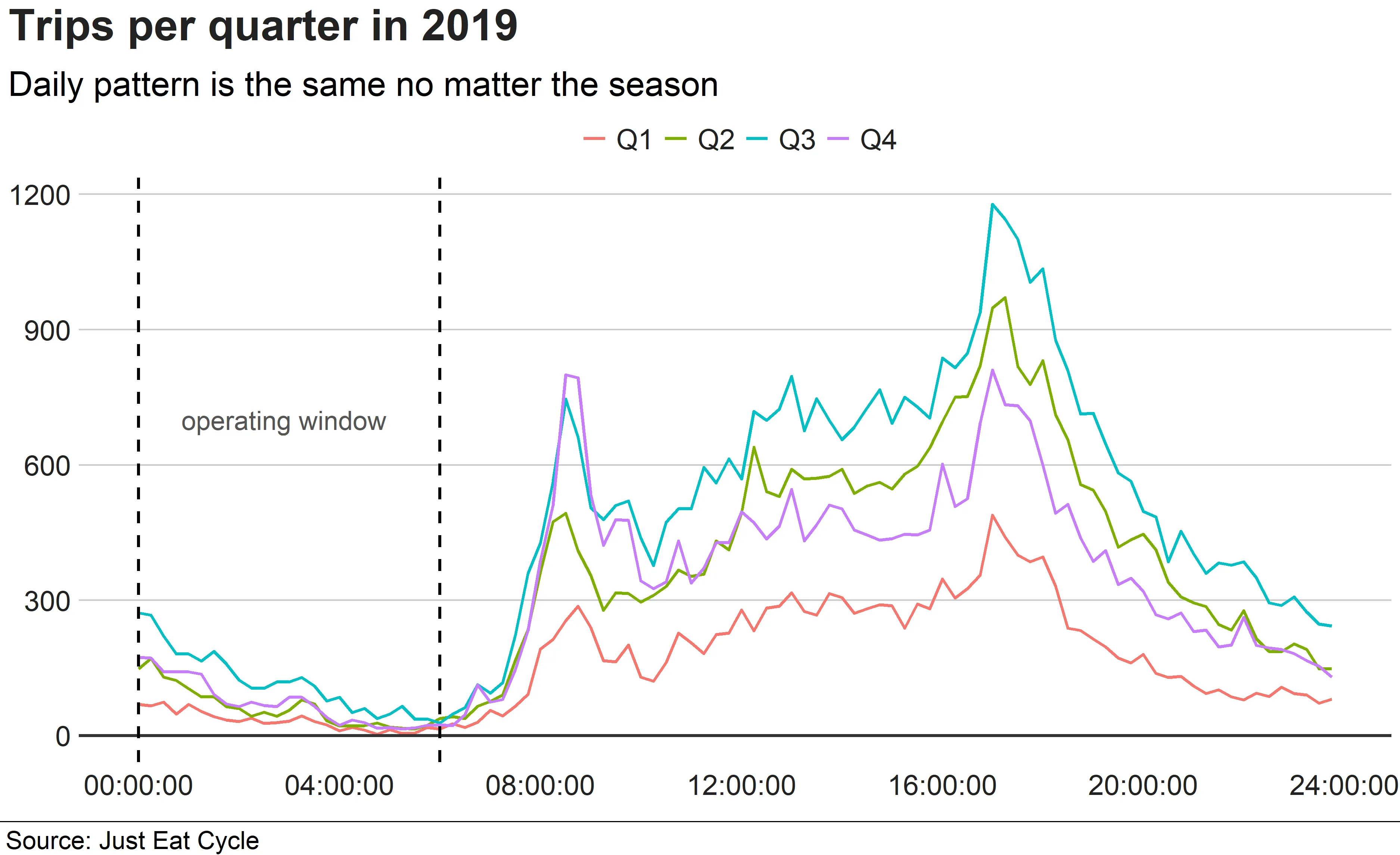
Average daily demand for bike trips by quarter in 2019.
Around 95 percent of trips happened between 06:00 and midnight, which hands you the answer to when to rebalance almost for free. Between midnight and 06:00 the network is effectively frozen: nobody is riding, so nothing you move gets undone five minutes later. That six-hour window became the operating constraint for everything that follows.
Seasonality
The second factor was the season of the year. While the shape of the daily pattern remained stable, the total demand varied strongly by month. In summer, usage was much higher, while in winter it fell significantly. To quantify this, I calculated seasonal factors by dividing the total demand in a month by the average monthly demand across the year. These factors allow demand to be scaled up or down depending on the time of year.
| Month | Factor |
|---|---|
| January | 0.464 |
| February | 0.456 |
| March | 0.639 |
| April | 0.825 |
| May | 1.382 |
| June | 1.030 |
| July | 1.200 |
| August | 1.673 |
| September | 1.405 |
| October | 1.217 |
| November | 0.983 |
| December | 0.728 |
This table shows that August demand was almost 70 percent above average, while January and February were less than half the average. These multipliers were later used to estimate station-level demand under different seasonal conditions.
Day of the week
Finally, day of the week. I expected this to be the easy one: busy Monday to Friday, quiet at weekends, commuters doing commuter things.
It was not there. Comparing weekdays and weekends month by month, the pattern kept reversing. In May weekdays were busier; in October it was the other way round. Some months peaked on a Saturday, others midweek.
So I dropped it and treated day of week as noise. That is worth saying out loud, because the tempting move is to keep a variable you were certain would matter and let the model sort it out. A predictor that flips sign depending on the season is not a weak signal. It is an invitation to overfit.
Mathematical model
Now to turn all of that into something a solver can chew on. What I want out the other end is concrete: which stations each van visits, in what order, and how many bikes it leaves at each one.
The catch is that there are two things worth optimising and they pull against each other:
- Minimise the time that stations spend completely full or completely empty, which reduces user satisfaction.
- Minimise the total time spent on repositioning, which reflects driver wages and van operating costs.
Either one is trivial on its own. Perfect availability? Send vans everywhere, all night. Zero cost? Leave the vans in the depot. The interesting solutions live in between, so both go into a single objective: penalties for stations left in a bad state, plus the time vans spend driving.
Modelling assumptions
To simplify the problem, I modelled rebalancing as a static problem carried out in the overnight window 00:00-06:00. During this period, demand is negligible and the system is effectively in a steady state. Vans can therefore work without interference from ongoing trips, traffic, or parking restrictions. The alternative would be dynamic rebalancing during the day, but this would be far harder to model and implement.
Additional assumptions included:
- Vans can pick up and drop off bikes within their capacity.
- Bikes at stations cannot exceed station capacity.
- The total number of bikes in the system remains constant.
- Drivers can also carry spare parts or batteries for e-bikes, with some extra time allowed for servicing.
Notation
| Symbol | Description |
|---|---|
| Set of stations, indexed | |
| Set of nodes (stations plus depot), indexed | |
| Set of vehicles (vans), indexed | |
| Number of bikes at station before repositioning | |
| Capacity of station | |
| Capacity of vehicle | |
| Number of bikes at station after repositioning | |
| Penalty function if station ends up empty or full | |
| Travel time between station and | |
| Total available time for repositioning | |
| Time to load and unload a bike respectively | |
| Binary variable, 1 if van travels from to , 0 otherwise | |
| Number of bikes carried by van when travelling from to | |
| Number of bikes loaded at station by van | |
| Number of bikes unloaded at station by van |
Objective function
The objective was to minimise the sum of penalties for stations plus the total travel time of vans:
The first term penalises stations that end up empty or full, while the second term accounts for the time taken to drive between stations.
Constraints
The model was subject to the following constraints:
The purpose of these constraints is to ensure the model behaves realistically. Constraint (1) keeps track of bikes at each station by accounting only for loading and unloading. Constraint (2) conserves inventory on vans, while (3) limits vans to their capacity. Constraint (4) enforces flow balance, ensuring vans that enter a station also leave it, and (5) prevents them from visiting the same station multiple times. Constraints (6) and (7) make sure vans do not pick up more bikes than available or overfill stations beyond their limits. Constraint (8) maintains conservation of bikes across the whole system, and (9) restricts rebalancing to the overnight time window. Finally, constraint (10) enforces non-negativity so that bike numbers, loadings, and unloadings are all feasible.
Computational approach
A model you cannot solve in time is an expensive way of writing down a problem.
Bike rebalancing is a mixed integer program, and MIPs grow faster than you expect. Add stations and vans and the search space expands at a rate that will happily eat a night of compute, which is awkward when the plan has to be ready before the vans set off.
To make the problem computationally tractable, I applied the following adjustments:
- Stations located close to each other were grouped into clusters, reducing the number of nodes in the model while still reflecting spatial patterns of demand.
- I assumed two vans were available for repositioning. This mirrored the actual scale of the Edinburgh scheme and reduced the number of routing variables.
With these simplifications, the problem remained realistic but could be solved within minutes on a standard laptop. This is fast enough to make daily rebalancing plans practical.
Example with 10 stations
To illustrate the model in action, I ran it on a simplified case with 10 stations across Edinburgh. The goal was to see how vans could redistribute bikes overnight so that no station was left completely empty or full by the morning peak.
Each station was assigned an initial inventory, a maximum capacity, and target reflecting historical demand. The model then decided how many bikes to load and unload at each location, and which routes the vans should take.
| Station | Initial bikes | Capacity | Target after repositioning |
|---|---|---|---|
| 1 | 12 | 20 | 15 |
| 2 | 5 | 15 | 10 |
| 3 | 18 | 20 | 15 |
| 4 | 8 | 15 | 10 |
| 5 | 20 | 25 | 22 |
| 6 | 6 | 15 | 10 |
| 7 | 14 | 20 | 15 |
| 8 | 9 | 15 | 10 |
| 9 | 11 | 20 | 12 |
| 10 | 17 | 20 | 16 |
Model results
The solver produced a feasible overnight plan using two vans. Each van performed a loop, picking up bikes from oversupplied residential stations and delivering them to undersupplied central ones.
| Van | Route (stations visited) | Bikes moved | Total time (minutes) |
|---|---|---|---|
| 1 | Depot → 3 → 7 → 2 → Depot | 25 | 110 |
| 2 | Depot → 5 → 10 → 6 → 4 → Depot | 30 | 130 |
Together, the vans redistributed around 55 bikes overnight, bringing every station closer to its target inventory. No station was left completely empty or over capacity, and the total time stayed within the 6-hour operating window.
Final thoughts
Ten stations is a toy. But the shape of the answer holds, and three things stood out.
Demand is far more predictable than it feels when you are standing at an empty dock at 08:40. The daily curve barely changes shape across the year, only its height moves, which means imbalances can be corrected in advance rather than chased in real time.
Two vans is enough. Not twenty. The overnight window is generous and the distances in a city like Edinburgh are short, so a small operation can keep the whole network honest.
The binding constraint is time, not capacity. Six hours between the last rider and the first one is the number everything else has to fit inside.
Edinburgh’s scheme has closed, but none of this was specific to Edinburgh. A bike share network lives or dies on whether people trust that a bike will be there. Rebalancing is the difference between a service you rely on and one you check the app for, sigh at, and walk instead.