Simulating a laptop assembly line in Simul8
A discrete-event simulation of a laptop assembly line in Simul8, using task-time distributions, model resource constraints, and staffing tests to identify bottlenecks and improve throughput.

Introduction
Assembly lines are a core part of modern manufacturing. They are used to produce everything from laptops to cars to food and medical equipment. The basic idea is to break the production process into smaller tasks, assign each task to a specific station or worker, and keep things moving. When the line is balanced, products flow efficiently. When it is not, delays build up, resources sit idle, and output slows down.
Understanding how an assembly line performs is important for any business that relies on one. Even small inefficiencies can lead to delays or higher costs when repeated across thousands of units. But figuring out what is actually causing those inefficiencies is not always straightforward. This is where simulation becomes useful.
In this post, I built a discrete-event simulation of a simplified laptop assembly line using real process data. The goal was to identify which steps limit performance and test changes that could improve it. By simulating the process before making real world changes, we can try ideas safely and see what actually works.
Input analysis
Before building the simulation, I needed to understand how long each task in the assembly line takes. Some of the task-time distributions were provided, but for the rest I was given historical data from 200 observations. My goal here was to estimate suitable probability distributions and test how well they fit the data.
Arrival process
For inter-arrival times, I assumed an exponential distribution. To estimate the rate, I used maximum likelihood estimation:
for data points . Substituting in our values for and , I arrived at . In order to determine the goodness of fit of this exponential distribution to our data I carried out a Kolmogorov-Smirnov test. I obtained a test statistic of which is smaller than the critical value of meaning that I could not reject the null hypothesis and can conclude that this distribution is reasonable.
Specific component assembly
For the keyboard and mouse placement task, I didn’t have a predefined distribution. I started by plotting a histogram and found that the data looked roughly normal. I calculated the sample mean and variance and used them to estimate the distribution as . To validate this, I ran a Chi-squared test, which gave a test statistic of Since this was below the critical value of , the normal distribution fit the data well.
And I followed a similar approach for other assembly tasks.
Simulation model
With the input distributions ready, I built the simulation in Simul8 to reflect the key logic of the laptop assembly process. I focused on a few core elements that had the biggest impact on flow and performance.
Orders arrived randomly and were only accepted if the number of laptops in the system stayed below a set limit. This WIP cap was important for keeping the system stable. Each accepted order was assigned an ID and split into two parallel branches, each representing a different part of the assembly.
Each task used the time distributions from the input analysis. Some tasks required specific workers or machines, and a few also depended on inventory being available. For example, aluminium cutting and hard disk placement were blocked if stock was too low, and inventory was tracked using global variables.
Once the subassemblies were complete, they were synchronised before moving on to final assembly and QA. The QA stage required two specific workers, and I treated this point as the end of production for measuring cycle time. Departure times and cycle times were recorded for each laptop.
To simulate material shortages, I included simple sub-models for aluminium plates and hard drives. When stock levels dropped below a threshold, an order was triggered and the system waited for a fixed delivery delay before replenishing. This helped capture the impact of material delays on system performance.
This structure was enough to observe how the system behaved under normal conditions and test different changes to see what improved it.
Below, I present a simplified version of the laptop manufacturing line used in the simulation, highlighting the main process flow and key synchronisation points.
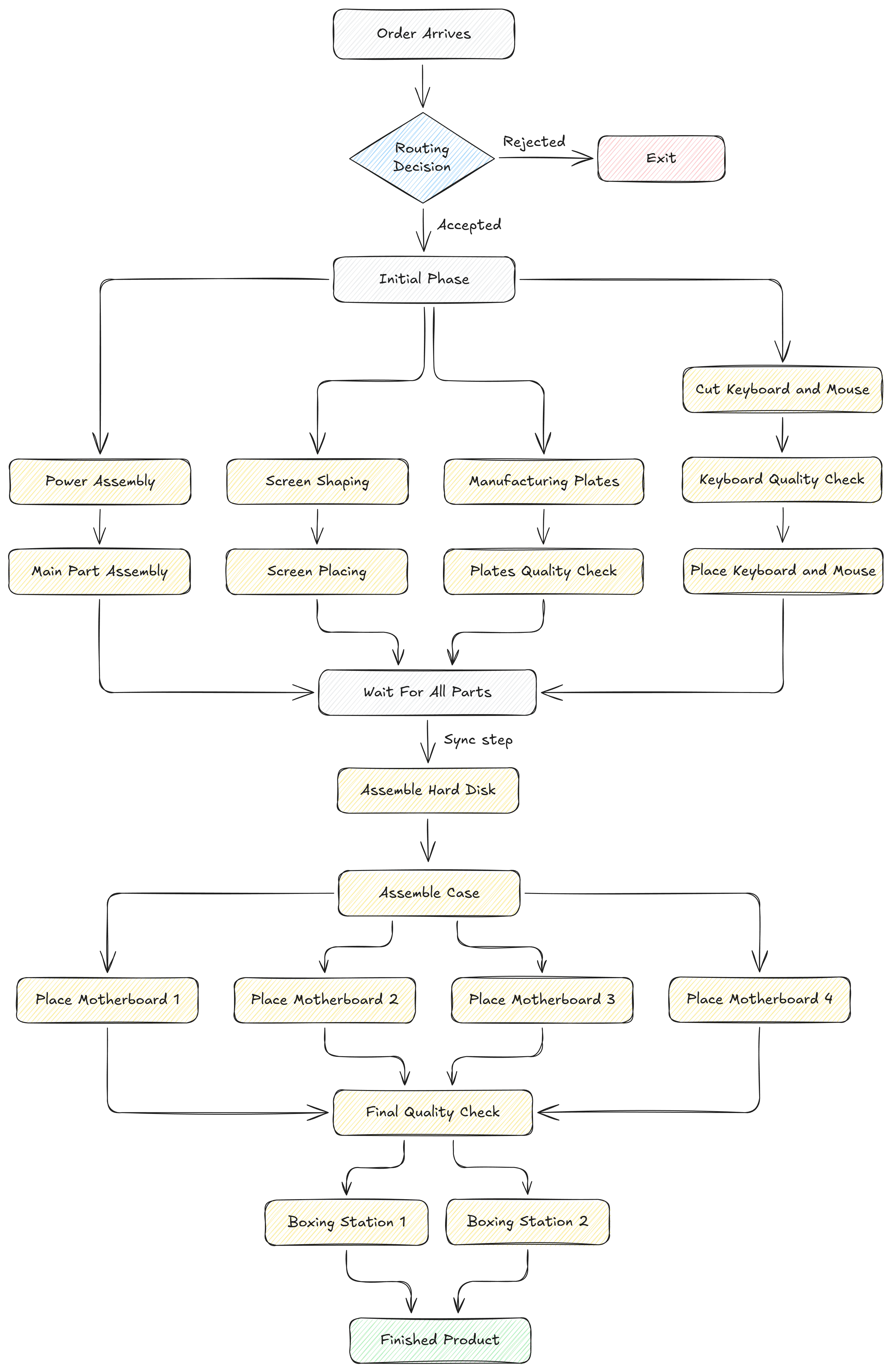
Laptop Simulation Overview
Output analysis
Once the model was complete, I ran the simulation over a one-year period and recorded key performance metrics. The main output I focused on was the cycle time, i.e. the time it takes for a laptop to move through the entire production process, from the moment the order is accepted until it passes the final quality check.
To calculate this, I time stamped each laptop at the start and again after it exited QA. I excluded the boxing stage from this calculation, since that happens after production is finished and can depend on unrelated batching delays.
Because the system takes time to reach steady state, I applied a “warm-up period” of 600 minutes before collecting any data. This was based on tracking a moving average of the last 10 completed cycle times. After the warm-up, I used batch means to calculate the average cycle time and other performance metrics. I also tracked queue lengths at each stage to see where work was building up.
The QA stage consistently had the longest queue, which suggested it could be a bottleneck. However, the average cycle time also showed periodic spikes that didn’t line up with QA delays. This pointed to another issue in the system, which I explore in the next section.
Recommendations
Based on the simulation results, I tested a few small changes to see what would improve performance. Some made a big difference, others had much less impact than expected.
The first and most effective change was increasing the reorder point for aluminium plates and hard drives. In the original setup, these materials were only reordered when stock dropped below 10 units. Combined with a 15-hour delivery delay, this caused parts of the line to stall and led to long cycle times. By increasing the reorder point to 20, I was able to reduce these delays significantly. The result was a clear drop in average cycle time, supported by a paired t-test over 50 batched runs.
The second change I tested was adding more QA workers. With only two workers at the QA station, a long queue had built up, which looked like a bottleneck. Doubling the number of QA workers brought the queue down from 80 minutes to under 2 minutes. However, this had almost no effect on the overall cycle time. That confirmed that QA looked busy, but it wasn’t actually the main constraint in the system.
Finally, I tested what would happen if I raised the WIP limit from 30 to 60. This allowed more orders into the system, which reduced rejections, but had no measurable effect on average throughput. It’s a useful change if the goal is to improve customer satisfaction or reduce lost orders, but it doesn’t help with delays unless something else is blocking the flow.
In short, the simulation showed that the most effective way to reduce cycle time is to address material availability. Fixing visible queues may help with flow smoothness, but doesn’t always move the key performance metrics.
Conclusion
This simulation helped me understand how a laptop assembly line behaves under realistic conditions, and where performance is actually limited. By modelling randomness in task times, resource constraints, and material delays, I was able to test changes in a controlled environment and see what really made a difference.
What stood out most was that the biggest delays were not caused by visible queues or busy-looking stations. They were caused by stockouts, simple gaps in material availability that halted production. Increasing the reorder points for key components had a much greater impact on cycle time than adding workers or changing WIP limits.
The model also showed that some problems are easy to misinterpret. QA had the longest queue, but speeding it up did not improve throughput. On the other hand, increasing the WIP limit helped reduce order rejections but didn’t affect delays unless the root cause, material shortages, was addressed first.
Overall, this post showed how simulation can be used to make better operational decisions. It gives us a way to test ideas, validate assumptions, and avoid spending time or money on changes that don’t deliver results.